Share This Page
| Home | | Mathematics | | * Maxima | | | | Share This Page |
(double-click any word to see its definition)
Those readers who have visited my Calculus tutorial will recognize this example — it is a common, well-understood differential equation with many real-world applications. For those who don't think about this stuff every day, a differential equation is one that expresses the relationship between a function and one or more of its derivatives. An example:
Statement
Let's examine the statements that describe the equation. In part (1) of the statement, we see that an unknown function y(t) is added to its derivative y'(t), which is scaled by two multiplier terms r and c.
In part (2) of the statement, an initial value is assigned to the function y(t). The meaning of this statement is that, when t = 0, y(t) = a.
Remember about differential equations that, unlike numerical equations, they describe dynamic processes — things are changing. Remember also that the derivative term y'(t) describes the rate of change in y(t).
Please think about this system for a moment. Let's say that the variable t represents time (although the equation doesn't require this interpretation). At time zero, the function y(t) equals a, therefore at that moment the derivative term y'(t) is equal to (b - a) / (r * c). Notice that y'(t), which represents the rate of change in y(t), has its largest value at time zero. Because of how the equation is written, we see that the value of y'(t) (the rate of change) becomes proportionally smaller as y(t) becomes larger. Eventually, for some very large value of t, the rate of change represented by y'(t) becomes arbitrarily small, as y(t) approaches the value of b, but never quite gets there.
Put very simply, this equation describes a system in which the rate of change in the value of y(t) depends on the remaining difference between y(t) and b, and as that difference decreases, so does the rate of change. As it happens, this equation is used to describe many natural processes, among which are:
This is by no means a comprehensive list of this equation's applications. But the statements for a differential equation are only the beginning, and not all differential equations have analytical solutions (solutions expressible as a practical function, one consisting of normal mathematical operations). Others require numerical methods and are only soluble in an approximate sense.
Let's see if Maxima can find a solution for this equation. Here are the steps:
eq:y(t)+r*c*'diff(y(t),t)=b; (equivalent to statement (1) above)
atvalue(y(t),t=0,a); (equivalent to statement (2) above)
sol:desolve(eq,y(t)); ("desolve()" is one of Maxima's differential equation solvers)
f(t,r,c,a,b) := ev(rhs(sol)); (assign the solution to a function)
(solved. "e" = base of natural logarithms)
Okay, we now have a function that embodies the solution to our differential equation. We can use it to solve real-world problems. Here's an example from a field in which I have spent a lot of time — electronics.
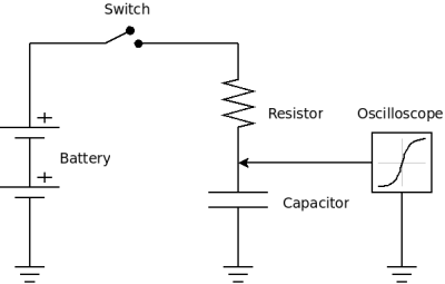
In this experiment, we have an electronic circuit consisting of a resistor and a capacitor. At time zero, we close a switch that connects our circuit to a battery, we then use an oscilloscope to measure the voltage on the capacitor over time (see diagram this page).
Here are the Maxima instructions to set up and graph the response of the described circuit:
r:10000; (10,000 Ω)
c:100e-6; (100 µf)
a:0; (ground voltage = 0)
b:12; (battery voltage = 12)
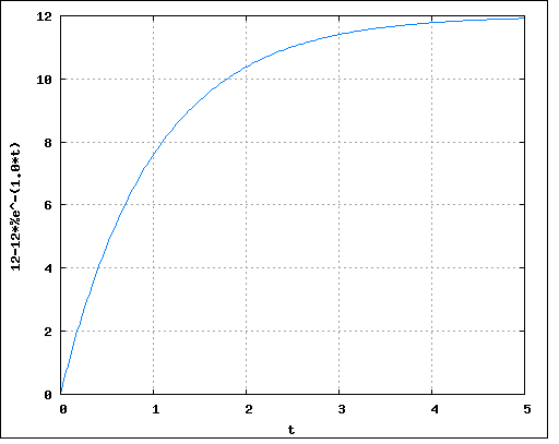
wxplot2d(f(t,r,c,a,b),[t,0,5], [gnuplot_preamble, "set grid;"], [nticks,12]);
I have to say this trace looks very familiar. Click here to download a Maxima instruction file for this problem and solution.
Okay, now let's move to a somewhat more complex differential equation that belongs in the same general class. In this equation, instead of a one-time event like throwing a switch that connects a circuit to a battery, we have a continuous waveform driving a system that could be an R-C circuit, or any natural system in which there is a path of resistance to the flow of something cyclical. I originally wrote this equation as part of a project to analyze the behavior of tides in channels that connect inland bays to the open ocean, but that is only one of many applications. Here again is a statement and a solution:
Statement
This equation has only one term, and no initial value. Let's submit this expression to Maxima and see what it comes up with:
eq:y(t)=-r*c*'diff(y(t),t)+m*sin(ω*t);sol:desolve(eq,y(t));
Okay, I see a problem with this solution — the group of terms at the right includes the familiar "e-t/rc" expression that appears in equations with defined initial values. But, because this equation describes a continuous process with no beginning and no end, we need to set the conditions at time zero in such a way that all times will be treated equally (and the right-hand subexpression will be eliminated).
After mulling this over, I decided the correct way to characterize the initial conditions would be to submit the right-hand expression as a negative value at time zero, which has the effect of preventing the assignment of a special time-zero value. Here is that entry and the outcome:
init_val:-(c*m*r*(%e^-(t/r*c))*%omega)/(c^2*r^2*%omega^2+1);atvalue(y(t),t=0,init_val); (a rather exotic initial value)
sol:desolve(eq,y(t));
f(t,r,c,ω,m) := ev(rhs(sol),fullratsimp,factor); (simplify, factor and declare a function)
(now this looks right)
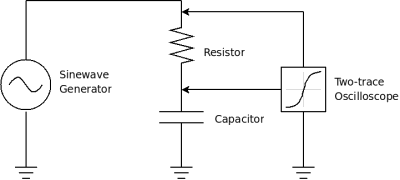
Okay, we now have a working embodiment of this equation, and it turns out this form has as many real-world applications as the earlier example. Here is another electronic example using an R-C circuit, but this time with a sinewave generator driving our circuit:
m:1;
f:440; (Hertz)
r:1000; (Ω)
c:0.05e-6; (µf)
ω:2*%pi*f;
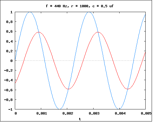
wxplot2d([sin(ω*t),f(t,r,c,ω,m)],[t,0,.005],[gnuplot_preamble, "unset key;set title 'f = 440 Hz, r = 1000, c = 100 uf'"]);
 -Signal Generator- -R-C junction-
Click here to download a Maxima instruction file for this problem and solution.
In case this virtual circuit design activity sounds exotic and unrealistic, I should say that modern electronic design has become increasingly dependent on this kind of virtual modeling, well in advance of any hardware prototyping. As computer software become more sophisticated, there is less reason to waste time and material experimenting at a workbench to discover that a design is or is not practical.
I found a rather exotic purpose for this differential equation up in Alaska. It turns out this equation applies naturally to the tide-driven movement of water into and out of bays connected to the ocean by narrow channels. The channel current resembles the current flow in the resistor in an R-C circuit, and the two waveforms in the diagram above resemble the timing and height of the water levels in an ocean-bay system (the blue trace represents the ocean water height and the red trace represents the bay). All one need do is establish time constants for the tidal system, which is nature's corollary to the time constants created by electronic components in an R-C circuit.
Of course, in nature things aren't so neat and predictable as in an electronic circuit, with an essentially perfect signal generator and electronic parts with precise values. But the two systems have a lot in common, and it is possible to model a bay's tidal heights with reasonable accuracy using this method.
| Home | | Mathematics | | * Maxima | | | | Share This Page |