

 Share This Page
| Home | | Ham Radio | | | | Share This Page |
An amazing intersection of mathematics, computer programming and radio
— All content Copyright © 2018, P. Lutus — Message Page —
Most recent update:

Figure 1: Virtual radio displaying the spectrum of an FM broadcast station
(double-click any word to see its definition)
Let me provide a context for my amazement at software-defined radio (hereafter SDR). My first electronic hardware designs predated the common availability of transistors — as a teenager I would inherit my neighbors' broken vacuum-tube TV sets and turn them into Ham Radio transmitters and receivers. Years later I designed solid-state electronics for the NASA Space Shuttle.
Then I decided to learn computer programming and wrote a very successful word processing program for the Apple II (Apple Writer). This personal history means I became familiar with electronic circuits and computers when they were both rather primitive.
In the days when I designed spacecraft electronics, I would begin with a mathematical notion that might or might not become a physical circuit. A large distance separated conception and realization, and the realization often bore only a slight resemblance to the conception. In those times it was slide rules to soldering irons.
All that has been swept away by events. It's not even a slight exaggeration to say we're witnessing a silent but widespread revolution that joins mathematics, electronics and everyday reality. Apart from abandoning many inefficient and dangerous things, like banks (replaced by blockchain) and cars driven by incompetents (replaced by self-driving cars), as a side effect this revolution shows the degree to which physical reality is innately mathematical.
This article covers available SDR hardware, software and configurations, but it also teaches a little radio theory and mathematics, the kind of mathematics we all need to understand to avoid being pushed aside in a more mathematically adept future society.
Figure 1 above shows what a modern radio receiver looks like. It can be tuned and adjusted by a pointing device, or by a network command, or by voice. It's important to understand that this is a virtual radio, not a physical one — it does what an old fashioned radio does (and more), but it's not part of physical reality. Essentially, the "radio" is defined by a set of mathematical equations designed to imitate an earlier, physical device.
This particular radio is displaying an electromagnetic spectrum created by a commercial FM radio station. The spectrum elements closest to the vertical red line (the "carrier frequency") carry music and announcements, what we expect to hear when we tune in a radio station with a conventional hardware radio. The two square blocks, located to the right and left of the central signal, carry special services provided by the radio station, like elevator music (i.e. "Muzak") and content directed toward special, niche audiences. Without a modern spectrum display we might never know about this special content.
RTL-SDR Device
Virtual radios like that pictured above work closely with a small, inexpensive external device — the hardware element most people associate with SDR — that accepts signals from a radio antenna and uses mathematics to convert the signals to a more useful form. Here's what such a device looks like:
")
Figure 2: Inexpensive SDR device
(There are many such devices available, I'm not endorsing this specific device.) In Figure 2, notice the two connections — at the left is an antenna cable that delivers radio-frequency signals from space to the device. At the right is a USB computer cable that delivers a processed form of the antenna input to the virtual radio shown in Figure 1.
I emphasize that, in the future, SDR devices like that shown above will be replaced by pure code and equations — no external hardware. Future computers will be so fast that they won't need dedicated modules to decode radio signals. But I digress.
The device shown in Figure 2 can decode signals from 24 MHz to 1.766 GHz. That covers a lot of territory — the FM broadcast band, many ham radio bands, all of modern TV broadcasting, public service (fire, police, etc.), aircraft, boats, "Family Radio Service" walkie-talkies, regional weather broadcasts and many other remarkable things (some of which I'm reluctant to reveal in a public forum).
NooElec Device
The above arrangement covers relatively high frequencies. To tune below 24 MHz with any reliability, one needs an additional device called an "upconverter" that works along with the basic SDR device. Here's what this special arrangement looks like:
")
Figure 3: SDR device plus upconverter needed for reception below 24 MHz
Unlike the earlier example in which I didn't want to seem to be endorsing a particular manufacturer's product, in this case I want to compliment NooElec.com on the upconverter module shown in Figure 3, which I regard as a first-rate product and superior to most competing products I've tested (apart from being a happy customer I have no connection with NooElec). It's not easy to design SDR hardware able to cover the spectrum from about 10 KHz (not a typo!) to 1.766 GHz, but (with some switch-throwing and offset frequency entries at the virtual radio) the arrangement shown in Figure 3 covers this entire range.
In Figure 3, an antenna suitable for HF reception (defined as the range from 3 to 30 MHz) is connected to the "Ham It Up" upconverter module (large connector at the left). The upconverter's output port is connected to the antenna input port of a typical SDR module (small pink cable), and the SDR module is connected via a USB cable (top center) to the computer hosting the virtual radio.
The upconverter covers the frequency range people usually associate with shortwave reception and Ham Radio activities, as well as the AM broadcast band (530 - 1700 KHz in the U.S.) and various special services located below the broadcast band including digital marine weather broadcasts and radiobeacons.
The cost for the combination of the upconverter and basic SDR module shown in Figure 3 is obviously greater than for the SDR module alone, but it's still reasonable.
As before, this is just a snapshot of current hardware at the time of writing (Winter 2018). In the future I expect development of a single, more economical external device that will cover the frequency range now requiring two connected devices as in Figure 3, but in the longer term this capability should be included in a personal computer's basic architecture.
HackRF One Device
")
Figure 4: HackRF One device
I mention HackRF One here because it has a feature that's unique among present SDR devices. In other respects HackRF One isn't a good choice for radio reception activities (and that's not its purpose — it's intended for radio-spectrum development work, not radio reception). But HackRF One has an interesting feature that deserves mention — it can transmit as well as receive wideband, complex (in the mathematical sense, i.e. I/Q inputs and outputs) user-defined RF signals.
My readers most likely understand what an audio recording consists of, and a video recording is just an extension of that idea with a wider bandwidth. We're now seeing a further extension of this idea into the RF spectrum, where a radio receiver can record wideband I/Q data (this terminology is explained below) from an antenna, save it to a file, then play it back — not as audio or video, but as a nearly perfect duplicate of the original radio transmission, same frequencies, same modulation. HackRF One is on a short list of devices able to do this.
In an experiment I set HackRF One to record a wideband radio spectrum that included the transmitting frequencies of two of my transceivers, set to different radio channels (HackRF One records I/Q data, not simple scalars — again, these terms are explained below). While recording, I activated one of the transceivers, then the other, then both transceivers at once — just to see if this combination of signals would confuse the recording process.
Then I let HackRf One play the recording back (in this case meaning transmit exactly what it had received). HackRF One wasn't confused in the least by this challenging test — it successfully played back the transceiver signals, including the moment when both transceivers were activated at once. I was amazed.
Again, if you're only interested in radio reception and want the most value for your money, my advice is to choose another unit. But if you want to experiment with RF signal recording and playback, do general engineering work and can afford this device, go for it.
Because so many people are writing and improving SDR software this section is likely to go out of date fairly quickly. But there are some worthwhile free SDR programs that deserve mention.
First, PLSDR — my own SDR program (free, open source, Linux and Windows compatible). This is an advanced SDR program that is in some ways better than the alternatives, and in some ways worse (I get to say stuff like that — I wrote it :) ). In the plus column is the fact that PLSDR is very easy to use — its user interface is carefully designed to make radio operation, tuning in particular, very easy. In the minus column is the fact that it won't run on a Raspberry Pi, one of my original goals. The project evolved in some very nice directions, but during the process it became too large to run on tiny computers (to my dismay). On that topic, Gqrx (described below) will run on a Raspberry Pi, so that might be a better choice if that ability is important.
Here's a picture of PLSDR in operation:

Figure 5: PLSDR User Interface (click image for full-size)
PLSDR supports a large number of computer radio devices and has been explicitly tested using three common examples. Also, the PLSDR Home Page includes a comprehensive tutorial on modern signal decoding methods, including some very educational JavaScript apps.
- SDR# (Windows only). This program is changing fast (new name: AirSpy) and may eventually be removed from the free category. I tried to get this program running on Linux — SDR# is written in C# and because there's a freeware version of Mono available for Linux, many C# programs can be run there. But at the time of writing, technical issues keep this from working. The Android version of this program is no longer free, but the Windows version is still free. Setup on Windows is overly complicated and requires a fair amount of technical skill.

Figure 6: SDR# User Interface (click image for full-size)
- Gqrx, Windows and Linux (including Raspberry Pi), free. A rather good cross-platform SDR virtual radio, in active development. This program can be successflly run on a Rasbperry Pi Model 3.

Figure 7: Gqrx User Interface (click image for full-size)
- CubicSDR, Windows and Linux, free. This program has some novel and ingenious interface features, it runs well on a desktop or laptop, but it's not suitable for use with a Raspberry Pi in its present form.

Figure 8: CubicSDR User Interface (click image for full-size)
There are many kinds of SDR hardware devices, each of which has special requirements. The above programs are able to work with the majority of available SDR devices by means of a wide collection of drivers and driver aggregation schemes. Because they're free, the reader can download and test them, decide which meets his/her requirements. But having said that, of the four programs described, I think PLSDR is the best choice for machines running Linux, followed closely by Gqrx, especially if the target platform is a Raspberry Pi (where my program can't function). For a Windows machine, same choices, but SDR# is compatible with that platform so it may deserve a look.
Let's take a closer look at the mathematical techniques behind SDR and virtual radios. To me personally, learning why something works is at least as interesting as knowing that it works.
Notice about Figure 1 (top of this page) that the horizontal scale has units of frequency, not time. The original signals are obviously distributed across time (the so-called "time domain"), but in a virtual radio we often see them as a spectrum (the "frequency domain"). This results from a conversion process called a Fourier transform, an ingenious mathematical way to convert signals from the time domain to the frequency domain. Here's an example:
AM FM Noise %
Figure 9: conversion from time to frequency domains
About Figure 9:
- Deselect "AM" (amplitude modulation) so a simple carrier wave is generated. Under these circumstances the resulting spectrum consists of one spectral line. This is equivalent to a single pure musical note.
- Increase the setting of the noise level slider and notice that one can still make out the frequency-domain spectral lines at the highest setting, even though the time-domain display has become unreadable. This is one of the many advantages of spectrum analysis — it reveals features that are lost in a time-domain display.
- The human ear is also a spectrum analyzer — like this example, it can pick out signals in the presence of high noise levels, and it can distinguish between frequencies with high precision.
- Deselect "AM" and select "FM" (frequency modulation). Notice that the FM spectrum is much more complex than the AM spectrum. There are many complex kinds of radio signals, but FM is high on the list of complexity.
- When both AM and FM modulation are deselected, the result is a continuous wave (CW). This simple waveform is sometimes used to send Morse Code dots and dashes, a robust method that remains the best choice when high noise levels or poor reception conditions prevent other methods from working.
The display in Figure 9 is generated by an algorithm called the Fast Fourier Transform (FFT), a method first conceived by mathematician Carl Friedrich Gauss, who in 1805 used it to compute the orbits of asteroids Pallas and Juno based on sparse observational data. The FFT was first used to avoid enormous amounts of tedious hand calculation, but as a computer algorithm it serves to make spectrum analysis lightning fast. Present-day virtual radios use the FFT to perform their spectral analyses.
It's important to understand about the Fourier Transform that it's bidirectional — one can convert from the time domain to the frequency domain and the reverse as well. This means we can design an impossibly complex waveform by placing desired spectral lines into an array meant to represent frequencies, converting the array from the frequency domain to the time domain, then perhaps use the resulting waveform to generate a radio signal with unique properties.
Don't be intimidated by the title of this section — vectors are just numbers with two (or more) components, sort of like "Walk North three steps, then East four steps, then look down. There's your dog." I bet if you were told how to find your dog like that, you wouldn't suffer an attack of math anxiety, and why should you? The described vector consists of two elements instead of one, so it can describe a location in two dimensions instead of one. No big deal.
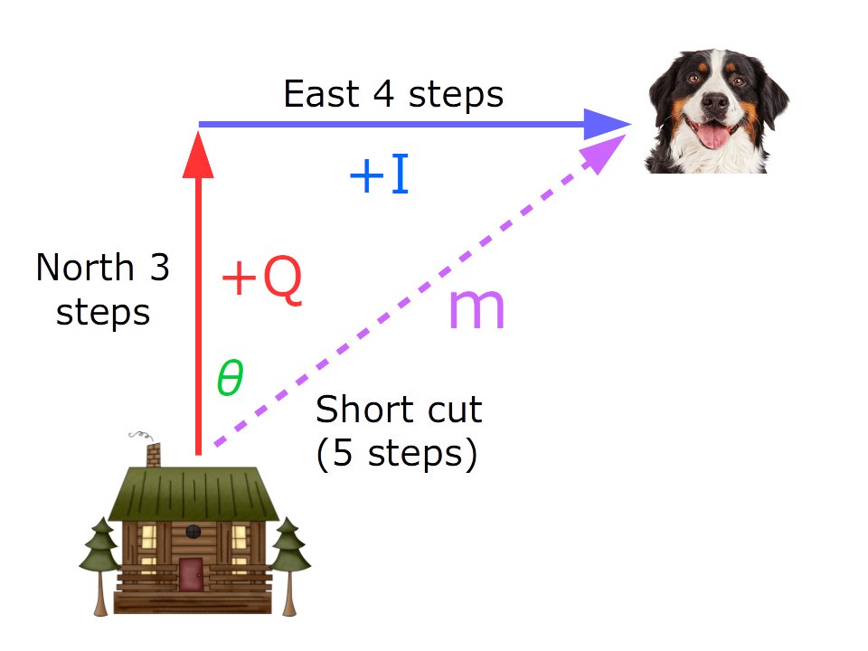
Figure 10: Numbers with two dimensions
Figure 10 shows a house and a dog, separated by a distance that can be expressed as a vector using Cartesian coordinates (i.e. X and Y, or equivalently I and Q), in polar coordinates, shown in Figure 10 as m and θ, or as the complex number I + Q$i$ (where $i^2 = -1$). Each of these forms serves a purpose, and each can be converted to another form when needed.
The terms I and Q actually have a meaning — I means "Inphase" and Q means "Quadrature" (more detail). I mention this because the use of I for the real component, and Q$i$ for the imaginary component, of a complex number seems perversely confusing, which is one reason I'm using colors to try to distinguish them.
A radio receiver that uses I/Q signal sampling has many advantages. Let's start by showing a generic (and somewhat unrealistic) I/Q mixer stage:
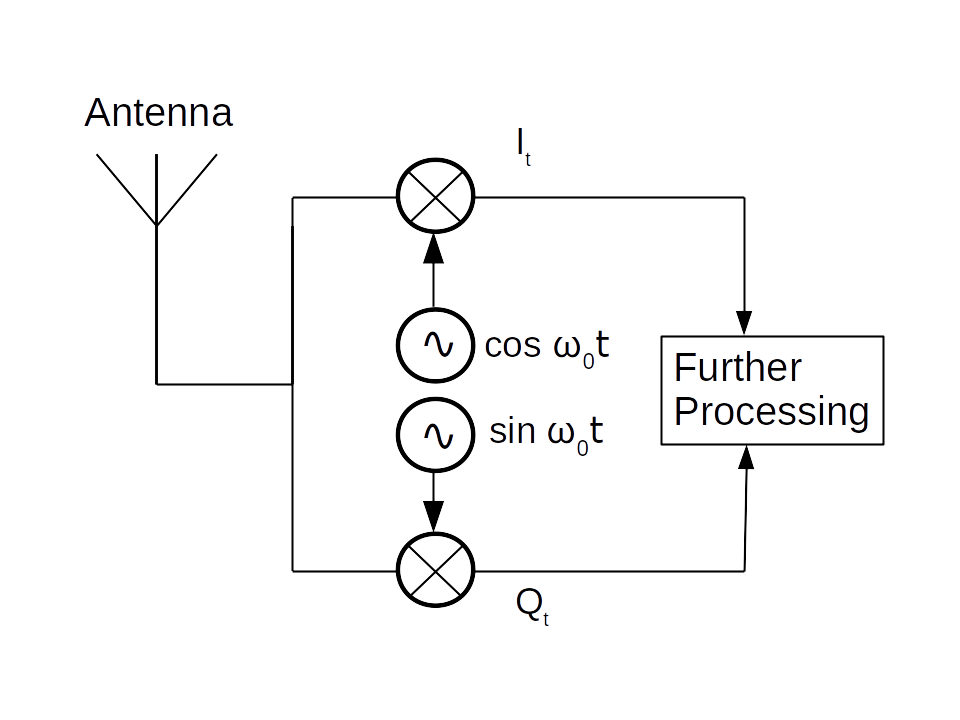
Figure 11: I/Q Sampling Diagram
For simplicity's sake Figure 11 shows an I/Q sampling configuration connected directly to an antenna (a source of analog data), but the same arrangement applies to a digital signal with small changes. In this diagram $\omega$ represents $2 \pi f$, $f$ being the local oscillator frequency. Because sin(x) lags behind cos(x) by 90° or $\frac{\pi}{2}$ radians, the I and Q components have this same phase relationship with respect to time — the provided Q oscillator reference differs from I by $\frac{\pi}{2}$ radians when pictured as a rotating vector, therefore the mixed Q signal component differs from I by $\frac{1}{4}$ of a circle, hence its name.
Before I/Q sampling became the norm, a typical radio receiver would implement only the upper half of Figure 11, the I component resulting from mixing the antenna signal with $cos(\omega_0 t)$. Now imagine the local oscillator is generating a signal at 1 MHz and the antenna delivers signals at 0.9 MHz and 1.1 MHz. In the earlier non-vector scheme, once the antenna signal was mixed with the local oscillator it would not be possible to distinguish between the two incoming signals — they would become indistinguishable to subsequent processing stages.
In an I/Q sampling system by contrast, the 0.9 MHz signal differs from the 1.1 MHz signal in a fundamental way — because the 0.9 MHz signal is below the local oscillator frequency (1 MHz), the resulting I/Q vector is rotating clockwise with respect to time (a so-called "negative frequency", a term explained below) while the 1.1 MHz signal's vector is rotating counterclockwise. These two vectors are easy to separate, which means the receiver can always distinguish between signals whose frequency is higher than, and lower than, the local oscillator, even signals having the same relative separation as in this example.
Another advantage of I/Q sampling is that the Fourier Transform responsible for (among other things) spectrum analysis benefits from the use of vectors. The transform can be carried out using scalars (single-component numbers) but information is irretrievably lost.
Yet another advantage to I/Q sampling is that the sampling rate can be half of what is required for a conventional sampling scheme (which requires a sampling rate of twice the highest frequency of interest) and produce the same results. Not to oversimplify, but this results from the fact that the I/Q mixer scheme shown in Figure 11 is collecting twice as much information from the incoming data stream, compared to an old-style scalar mixer. This means a device with a clock rate constraint can acquire more data and a wider bandwidth by using I/Q sampling.
This is just a short list — there are many other advantages to I/Q sampling, but increasingly technical and therefore not suitable for this introductory article.
Figure 12 is a JavaScript applet that lets you explore the behavior of I/Q sampling schemes and their consequences. Below the applet are instructions and a list of experiments to try.
Figure 12: Interactive JavaScript I/Q exploration appletInstructions and suggestions for Figure 12:
- Enable real-time animation by selecting the "Animate" checkbox.
- Rotate the 3D graph by dragging your pointing device on its surface, zoom with your mouse wheel.
- Try enabling/disabling the provided options and entering different frequences and rates.
- A set of example Configuration State buttons is provided to show various aspects of I/Q sampling:
- The State A example forces the 3D display into a flat, old-style 2D oscilloscope display without I/Q sampling, just to provide a contrast with the newer methods. After clicking "State A", rotate the graph with your pointing device to bring the I/Q elements back into view.
- The State B example shows the phase relationship between I and Q for the case of a positive frequency. In this case, Q lags I by 90° or $\frac{\pi}{2}$.
- The State C example shows the phase relationship between I and Q for the case of a negative frequency. Notice that the only change between this example and State B is in the phase of Q, which tells us that an old-style mixer without I/Q sampling would not be able to distinguish between a positive and negative frequency.
- The State D example shows a time animation of a negative frequency vector. To see the contrast between negative and positive frequency, change the sign of the carrier frequency and notice that the vector's direction of rotation reverses.
- Remember that the meaning of "clockwise" and "counterclockwise" depends on one's point of view. For example, the default animation appears to show a clockwise rotation for a positive frequency, but this is so only because of the default graph point of view, located to the right of the graph. But the clockwise/counterclockwise convention applies only when looking toward a future time, i.e. from a position at the left of the graph, as in the State D example.
- To speed up / slow down the animation rate, increase / decrease the value of "Anim. Step."
- To see this display in true 3D, select the "3D" checkbox and grab a pair of red/cyan "Anaglyphic" 3D glasses.
- It's my hope that this applet will provide a memorable visualization of the details of I/Q sampling, to help the reader acquire an intuitive sense of how and why it works.
Vector Conversions
Three kinds of two-dimensional vectors were introduced above — Cartesian (x and y or equivalently, I and Q), Polar (magnitude $m$ and angle $\theta$) and Complex ($I+Qi$). Each of these can be easily converted to the other forms as required:
- Cartesian to Polar: $m = \sqrt{x^2+y^2}$, $\theta = \tan^{-1}(\frac{y}{x})$
- Polar to Cartesian: $x = m \cos(\theta)$, $y = m \sin(\theta)$
- Cartesian to Complex: $x,y$ -> $x+yi$ (remember that $i^2 = -1$)
- Complex to Cartesian: $x+yi$ -> $x,y$
- Polar to Complex: First convert Polar to Cartesian, then Cartesian to Complex.
- Complex to Polar: First convert Complex to Cartesian, then Cartesian to Polar.
The above Complex <-> Cartesian conversions only apply to the simplest expressions, i.e. a pair of simple scalar quantities. For other conversions, the rules are ... well ... more complex.
Angle Units
Students who have worked primarily with calculators and who are getting into programming, need to be aware that the default trigonometric angular unit is the radian, not the degree. Behind the scenes, trigonometric functions all require arguments to be expressed in radians. So:
Degrees ($d$) to Radians ($r$): $r = d \frac{\pi}{180}$
Radians ($r$) to Degrees ($d$): $d = r \frac{180}{\pi}$
| Home | | Ham Radio | | | | Share This Page |