Home | Ruby | Graphinity |     Share This Page
Graphinity: Graphing in Depth
All content Copyright © 2008, P. Lutus

Version 2.4, 11/02/2008

Source package: graphinity.zip (27.5 KB)

Introduction | Getting Started | 2D Example Graphs | Error Recovery
3D Example Graphs | Anaglyphic 3D | Ruby-Specific Equation Syntax
Exporting Images | Supported Mathematical Functions | Revision History

(double-click any word to see its definition)

Introduction

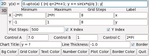
Graphinity's 2D display
(click image for full-size)

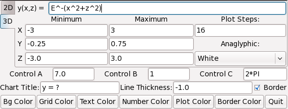
Graphinity's 3D display — best viewed
with anaglyphic glasses ()
(click image for full-size)
NOTE: Be sure to visit Graphinity Online, an interactive JavaScript version of this program.

This is the latest in a series of graphing programs I have written over about 30 years. Because Ruby development moves along so quickly, this project required much less time than its predecessors.

Graphinity is a graphing application that produces graphs of user-entered mathematical functions in 2D, perspective 3D and anaglyphic 3D (meaning with visible depth — see the first image on this page). The only desirable accessory is a pair of anaglyphic glasses, with red and blue lenses. Graphinity is free and is released under the GPL.

Some miscellaneous notes:

  • Graphinity is a perfect example of a program that deserves to be written in Ruby. The program doesn't need to run particularly fast, Ruby testing and development time is very fast, and I expect the program to need revision in the future, something Ruby makes easy.

  • On the downside, version 1.0 of this program used the Qt graphics libraries, but in the interim Trolltech decided to release a new version of Qt without providing either support for legacy applications or a practical way to upgrade existing applications. Consequently, after only two years, Graphinity and some other of my applications were rendered completely inoperable. I personally will never use Qt again. The new version uses the GTK+ libraries.

  • Newer versions of Graphinity have some advanced user-interface features. One is the fact that you can change most numerical entries by spinning the mouse wheel over them — this allows you to interactively change a graph's appearance by spinning the mouse wheel. The other feature is three user-defined variables (a, b, and c) — you can add the variable names to an equation or a scaling control and then spin your mouse wheel over the control variable to control things. This greatly improves the interactive nature of graphing activities.

Getting Started
To run Graphinity, you will need Ruby and the GTK+ utility library. Like Graphinity itself, both these resources are free.

Here is a capsule summary of Graphinity:

What it is: A graphing program for students and others who need an easy way to create graphs of mathematical functions in 2D, perspective 3D and anaglyphic 3D. The program is highly interactive and invites experimentation. The user can export the resulting graphs into any clipboard-enabled application.
Written using: Ruby 1.8.6. Click here to see the program's Ruby listing.
Requires: The GTK+ library, version >= 2.0 (Linux/Windows), and Ruby, version >= 1.8+ (Linux/Windows). Both GTK+ and Ruby are free, cross-platform and open-source.
Optional, very desirable: Anaglyphic glasses () to see the 3D effects.
Source: Ruby interpreter files: graphinity.zip (27.5 KB).
License: GPL.
To run Graphinity, download and install the language packages listed above (Linux users can do this with their favorite package manager), then download and unpack the Graphinity zip file into any convenient directory. Run Graphinity from a command shell (Linux: "./graphinity.rb", Windows: "graphinity.rb"). Later on you may want to create a platform-specific shortcut for the executable.

There is a help window in Graphinity that covers the basics, most of which will be described here also. Basically the user types a mathematical function for graphing and presses the Enter key to create the graph. Beyond this, the user can scale the graph to suit the entered expression, exercise various display options, and copy the resulting graph to the system clipboard.

2D Example Graphs
Let's cover two-dimensional graphs first, the sort of graph one might want to include in an article or Web page. Graphinity first runs with a default set of values, including this 2D graphing equation:


y(x) = e-x2
            

It would be nice if this equation could be entered into Graphinity just as shown, but Graphinity requires a sort of ASCII shorthand that the user may find familiar:

y(x) = E^-x^2
            

This is the default equation, it will be present when Graphinity is first run, but for this example, type it in and press Enter to see the resulting graph. In passing, let me add that uppercase "E" is a program constant equal to the base of natural logarithms (2.71828182845905 ...), one of two constants predefined in Graphinity (the other is PI).
NOTE: Don't type the beginning of the equation (y(x) = ) into Graphinity. That part isn't needed and it will cause an error.


Graphinity 2D control panel

Graphinity 3D control panel
Now experiment with some equations of your own, and notice that some require you to scale the display to make the entire graph visible. That is the purpose for the X and Y minimum and maximum value entries. For example, let's say you've entered this equation:

y(x) = sin(x)
            

To show this graph, you may want to change the Y minimum value to -1.0, to allow for the fact that sin(x) has a range of -1.0 to 1.0. You may also want to change the X input value range: minimum = -PI and maximum = PI, to show one complete cycle. Yes, Graphinity allows you to enter things besides numbers into most of its value entry windows, not just the equation window. Just to show how this feature might be useful, enter this data:

Equation: y(x) =  x^2
X minimum -sqrt(2)
X maximum sqrt(2)
Y minimum 0.0
Y maximum 2.0

Because of how the X limits have been set up, the resulting graph reaches maxima of exactly 2.0 at the X range extremes.

Graphinity allows you to pluck specific values from a graph. Here is an example of this feature:

Equation: y(x) =  m=100;sd=15;(1+erf((x-m)/(sd*sqrt(2))))*50
X minimum 50
X maximum 150
Y minimum 0
Y maximum 100
To save time, just copy the above equation from this Web page and paste it (using Ctrl+V) into the Graphinity equation window. This example uses the Gaussian error function erf(x) to display a distribution of I.Q. scores within a hypothetical population with a mean I.Q. of 100 and a standard deviation of 15. I want to emphasize about this example that it has very little to do with reality (I.Q. testing is not at all reliable), I just think it's a nice example.

You may want to enlarge the graph for this exercise — click the "Display" tab, and also maximize the program window if you want. This improves your ability to sample specific graph values.

Having entered the values above and graphed the equation, put the mouse cursor on the graph and press the left mouse button. Drag the mouse around and you will get the idea — the entered equation has produced a curve of statistical results, and you can use your mouse to get particular results from the function. For example, move the mouse until the X value is about equal to 115 and read the resulting Y value of 84.1345, more or less. This is a way to sample a function in an approximate way — approximate because the mouse resolution is limited — and to gain an intuitive sense of how a function behaves (this result means 84.13% of people in our hypothetical population have an I.Q. of 115 or less).

This example is a generic plot of a standard distribution, with assigned values for mean and standard deviation. It's too bad it alludes to such a disreputable part of human psychology (I.Q. testing), and I want to say again that it's just a hypothetical example.

By allowing the declaration of variables, this example reveals the Ruby underpinnings of the equation processor. Even though Graphinity appears to be processing pure mathematics at first glance, one quickly realizes it accepts a fair amount of Ruby-specific syntax, like variable declarations. But I have made one change — Ruby won't normally accept "^" for raising a number to a power, but I have translated this symbol internally to allow Graphinity to accept this common mathematical convention.

Play with some of the other controls in the 2D control set, like "Grid Steps", "Label" and "Numbers", which govern various visual aspects of the graph. Also notice the "Grid:" control at the lower left — this control determines the appearance of the graph's grid lines. And finally, notice the color buttons at the bottom of the control panel. These allow you to choose colors for most parts of the graph.

Error Recovery
When you exit, Graphinity saves everything — the program window size, your entered numbers and color choices, the most recent equation, everything. I have tried to make Graphinity as friendly and coöperative as possible. But, because of this policy of saving everything, it's possible to make a bad entry and not be able to recover, so here is how to make Graphinity start over with the default program values:

  • Exit Graphinity.
  • Locate your user home directory.
  • Within your home directory, locate a program data directory named ".Graphinity".
  • Delete this directory, or delete the file it contains, "Graphinity.ini".
    NOTE: The Graphinity help page will display the exact location of your home directory and of the file you need to delete.
  • Run Graphinity again.
3D Example Graphs
There are many mathematical equations better presented and viewed in three dimensions. Graphinity has a rather sophisticated equation renderer that will produce both perspective and anaglyphic 3D images.

Click the tab marked "3D" at the left center of the control panel. The default 3D equation should be on display:

Equation: y(x,z) =  E^-(x^2+z^2)
X minimum -3.0
X maximum 3.0
Y minimum -0.25
Y maximum 0.75
Z minimum -3.0
Z maximum 3.0

Some words of explanation. The reader will notice an additional variable in this section — "Z". Remember that in equation graphing, X and Y may refer to arbitrary quantities, but they also can refer to space dimensions for graphing purposes. In that sense, X is the left-right dimension, Y is up and down, and Z is, well, toward and away, so to speak. These dimensions are all orthogonal (all at right angles to each other), and three such values are needed to define a point in 3D space.

Remember this simple rule. In the Graphinity graphing window, X refers to the horizontal axis, Y refers to the vertical, and Z refers to the dimension of depth or distance. Later on, we'll be rotating the entire 3D graph, meaning these terms are relative once you have spun the graph around.

In Graphinity's 3D space, both X and Z set the equation's input range as well as establish the display scale for these dimensions, while Y sets the vertical display scale as it does for 2D graphs.

The examples that follow, and 3D graphing in particular, is rather demanding on a computer's processing power. The most significant determining factor for rendering speed is the number of 3D plotting steps chosen by the user. If you find the update speed is unacceptable, the best solution is to decrease the "Plot steps" entry. The overall update speed is proportional to the inverse square of this number.

First, before we leave the default equation listed above, put your mouse cursor within the graph window, press the left mouse button, and move the mouse. In the 3D graph, mouse motions rotate the graph in 3D space — move the mouse horizontally to spin the graph around, and move the mouse vertically to flip the graph over. Finally, move the mouse wheel to zoom in and out.

Now for a few example graphs. Here is one that places rather heavy demands on the computer's processing speed:

Equation: y(x,z) =  q=(x^2+z^2);E^-q*cos(q*3)
X minimum -2.0
X maximum 2.0
Y minimum -0.25
Y maximum 0.75
Z minimum -2.0
Z maximum 2.0

This example superimposes a cosine wave on the original Gaussian curve, a graph sufficiently complex that it is almost a requirement to increase the number of plot steps beyond the default value of 16. Remember again that the plotting speed declines as the square of this number.

While rotating this graph around, the reader may find it difficult to visualize it accurately in three dimensions using only the default perspective display. This is true for a large number of relatively complex mathematical functions, which is why Graphinity can produce anaglyphic 3D.

Anaglyphic 3D 
Anaglyphic 3D uses a special pair of glasses, with red and blue lenses, to give the viewer two different views of an object, one for each eye, which produces the illusion of depth. To provide a bit more detail, the reason we see depth in the world around us is because our eyes deliver two views from slightly different angles. Any technique that can deliver two properly crafted images to our left and right eyes can produce the illusion of depth. The anaglyphic method can do just that, and the only extra cost to the user is a pair of special, relatively inexpensive, glasses with red and blue lenses.

To activate the anaglyphic feature in Graphinity, go to the drop-down box labeled "Anaglyphic:" and choose one of the options "White" or "Black". Each of these options creates an anaglyphic 3D view of the graph, one with a white background, one with a black background. The white background is particularly suited to image export (see examples on this page), in particular if the anaglyphic image might be printed on a color printer. Such a printed copy will retain the anaglyphic 3D effect if the printer renders red and cyan colors with reasonable fidelity.

Here's another example equation, one that is also difficult to picture without the anaglyphic feature:

Equation: y(x,z) =  sin(x) + sin(z)
X minimum -PI
X maximum PI
Y minimum -2
Y maximum 2
Z minimum -PI
Z maximum PI

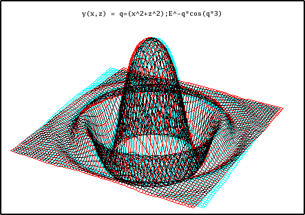
This equation is displayed in the first graphic on this page. Try rotating this graph, both with and without the anaglyphic feature, to see how much easier it is to visualize using anaglyphic 3D.

Ruby-Specific Equation Syntax
Some examples have already been presented that rely on Ruby-specific aspects of the equation processor, here is another. Enter this equation into the 3D panel:

Equation: y(x,z) =  [ cos(x), cos(z) ].max
X minimum -PI*3
X maximum PI*3
Y minimum -2
Y maximum 2
Z minimum -PI*3
Z maximum PI*3

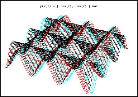
I call this equation "the waffle" for reasons that should be obvious. The idea of this equation (or, more correctly, Ruby function) is that two trigonometric values are generated independently, and the largest value between them is chosen for each point on the graph. As a result, we see two crossed patterns of waves, one on the X axis and one on the Z axis.

Exporting Images
Exporting your work is very easy — just right-click the graph and select "Copy Chart to Clipboard." Open the destination application and paste. I chose this way of exporting images because I would otherwise have had to choose which graphic formats to support, and then I would have had to actually support them. I decided a clipboard copy would be more useful overall.

If you intend to print the graph, either 2D or 3D, be sure to export your work with a white background. I have even had some success printing the anaglyphic images using a color laser printer. The best printers only approach the color rendering fidelity of an average modern computer monitor, but it's interesting to see the expression on people's faces when you hand them a piece of paper and a pair of anaglyphic glasses.
Supported Mathematical Functions
Graphinity basically supports the function set provided by the Ruby Math class. Also note again that Graphinity will acept the "^" caret character to signify raising a number to a power. This is a character Ruby normally reserves for a different purpose.

All trigonometric arguments should be provided in radians.

acos(x) Arc cosine of x.
acosh(x) Inverse hyperbolic cosine of x.
asin(x) Arc sine of x.
asinh(x) Inverse hyperbolic sine of x.
atan(x) Arc tangent of x.
atan2(x,y) Arc tangent, two arguments, approximately atan(y/x), but with quadrant resolution.
atanh(x) Inverse hyperbolic tangent of x.
cos(x) Cosine of x.
cosh(x) Hyperbolic cosine of x.
erf(x) Error function of x.
erfc(x) Error function complement of x.
exp(x) E raised to x, e.g. E x . E = base of natural logarithms.
hypot(x,y) Hypotenuse of x and y, that is, sqrt(x^2+y^2).
log(x) Natural (base E) logarithm of x.
log10(x) Base 10 logarithm of x.
sin(x) Sine of x.
sinh(x) Hyperbolic sine of x.
sqrt(x) Square root of x.
tan(x) Tangent of x.
tanh Hyperbolic tangent of x.
Revision History
Here's that download link again: graphinity.zip (27.5 KB)

  • Version 2.4 11/02/2008. Increased the number of user variable controls to 3 (a, b, and c) for increased interactivity, updated help file.
  • Version 2.3 11/01/2008. Added the mouse-wheel control feature to all numerical fields, fixed a minor bug.
  • Version 2.2 10/20/2008. Added an interactive control variable that can be included in an equation or a scale entry.
  • Version 2.1 10/19/2008. Cleaned up some minor bugs, updated help file.
  • Version 2.0 10/18/2008. Recovered application by eliminating any use of Qt libraries.
  • Version 1.0 09/25/2006. Initial Public Release.
 

Home | Ruby | Graphinity |     Share This Page